함수근사와 관련된 모델에 대하여 통계적관점, 학습 behavior 관점으로 알아보자.

Regression Problem (회귀문제)

1. parametric or non-parametric model
   • prametric estimation : f의 functional form을 아는 상태
   • non-parametric estimation : f의 functional form을 모르는 상태. 따라서 f의 functional form을 만들어야함.
2. linear or non-linear model
3. simple or multiple regression
   • simple regression : f is a univariate function
   • multiple regression : f is a multivariate function

보통 non-linear / multiple regression model이 일반적이다.

A simple linear regression model

위와 같은 linear regression model이 있다고 할때

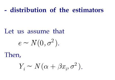
노이즈 e와 근사값 Yi는 위와 같은 분포를 따른다.
=> an estimator of Yi(Yi의 추정량.근사치) : Yi hat = A+Bxi (A는 알파의 estimator, B는 beta의 estimator)
=> sum of square residuals(errors) - SSR

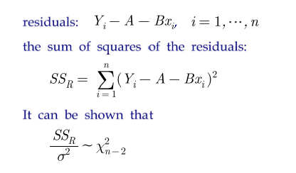
=> solution을 알려면? SSR 미분해서 0인곳. (꼭지점) –> SSR을 A와 B로 편미분하여 각 방정식이 0인것을 고른다.

some notations

식이 자꾸 복잡해지니까 앞으로 아래와 같은 notation을 사용한다.

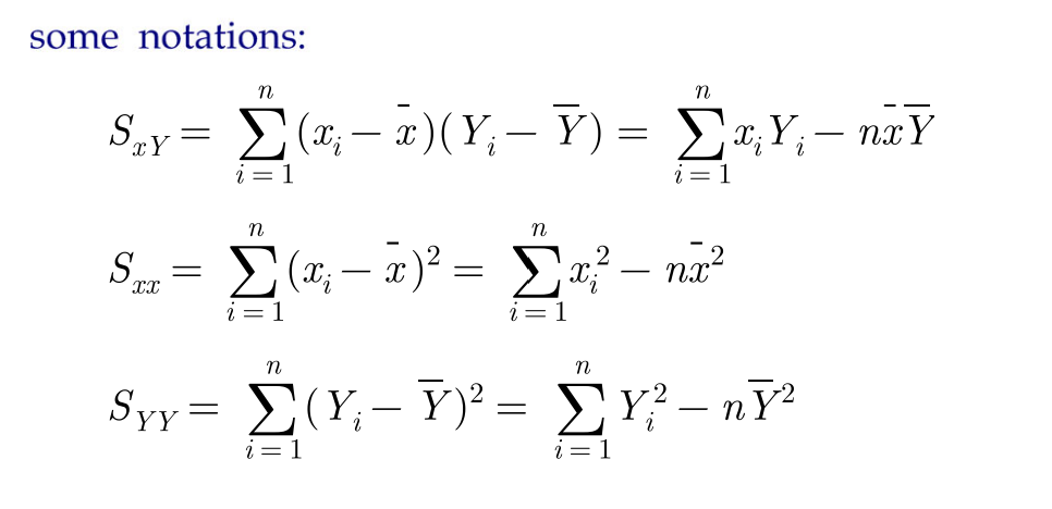
=> 이 nottaion을 사용하면 SSR을 A로 미분했을시 => A = Y - Bx, B = Sxy / Sxx
(앞으로도 계속 이 notation은 사용됨)

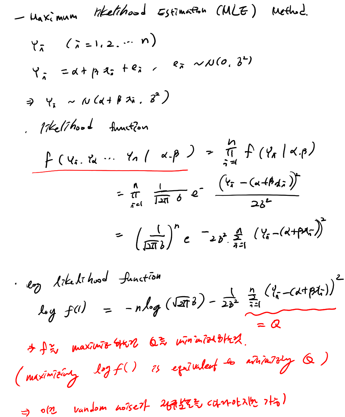
Maximum likelihood Estimation (MLE) Method

(글씨개판..)
최대 우도(가능도) 추정법
어진 Dataset의 발생 가능성(Likelihood, 우도)이 가장 높은 모수를 추정하고, 이를 바탕으로 최적의 f를 도출하는 방법.

chi-square distribution (카이제곱분포)

Zi ~ n(0,1) i= 1,2,…n
Zi are in dependent random values
=> X = summation Zi/^2 ~ X^2 n
카이제곱분포 wit n degrees of freedom
E[X] = n
Var(X) = 2n

estimation of sigma square (o^2)

SSR / o^2 ~ X2n-2 (카이제곱분포를 따른다)
E[SSR/o^2] = n-2 —– > o^2와 n-2는 interchange 가능
E[SSR / (n-2)] = o^2
bias of parameter
d : an estimator of parameter theta
b theata (a) = E[d] - theata => b theta (d) = 0; that is E[d] = theta
=> an estimator of sigma square = an unbiased estimator of sigma square.
–> unbiased estimator라는것은? 샘플이 많아질수록 진짜값에 근사하게된다는 뜻.
–> c.f biased estimator는 편향된 estimator라는뜻.

Distribution of B

B = Sxy / Sxx
E[B] = b
Var(B) = o^2 / Sxx
B ~ N(b, o^2 / Sxx) 정규분포를 따름

Distibution of A

A = Y - Bx = 1/n summation Yi - Bx
E[A] = a
Var(A) = o^2 / Sxx * 1/n summation x^2
A ~ N(a, o^2 / Sxx * 1/n summation x^2)

normalized form (정규화)

standard normal. 이 모양을 가지고 계속 다루게된다.

T-distribution (T 분포)

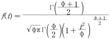
f(t)를 가진 분포. 자유도가 높아질수록 정규분포에 가까워진다.

Confidence interval(신뢰구간)

Xi ~ N(M, o^2)
sample mean X bar = 1/n summation Xi ~ N(M, o^2/n)
an estimation of M => xbar - M / o / root n ~ N(0,1)
우리는 모집단의 평균 뮤(M)를 모르니까..
이걸 T분포로 풀어봐서 1-a의 확률로 M가 어디에 위치하는지를 풀어봄..
accuracy를 이야기할때 이 length로 이야기함.
high accuracy => small L (length)

Confidence interval for the mean response of Y

for the given input x0, Y0 = a + px0 + e, e ~ N(0, o^2) -> E[Y0] = a + bx0 hat Y0 = A + Bx0 -> E[hat H0] = E[A+Bx0] = a + bx0

=> Var(A + Bx0) = o^2 ( 1/n + (x - x0)^2 / Sxx) tn-2 분포로 신뢰구간을 구할수있다. => a for 100 (1-a)% confidence interval for a+bx0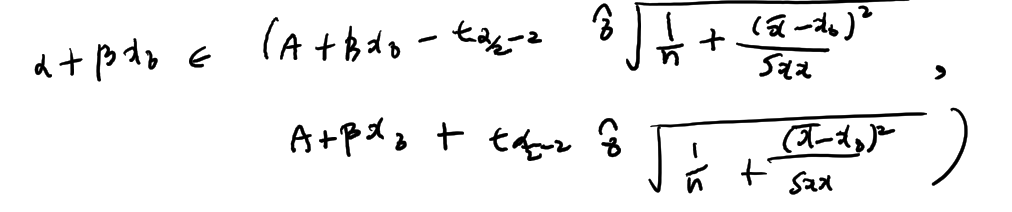

=> center에서 estimation의 accuracy가 제일 높다..

Coefficient of Determination (결정계수)

R^2 = Syy - SSR / Syy = 1 - SSR / Syy
R^2 는 에러variation과 Y의 variation값을 비교한것. 0 <= R^2 <= 1
near 1 : a good fit for the data near 0 : a poor fit for the data

e.g.
Syy = 38.521, SSR = 1.497
=> R^2 =.497 / 38.521 1 - 1 = 0.961
=> 이 말의 뜻은 Y variation의 96%를 이 regression model이 설명해준다는것.

Analysis of Residuals

우리가 세운 가설이 잘맞는지 분석할필요가있음. Yi = a + bxi + ei ~ N(a+bxi, o^2) hat Yi = A + Bxi ~ N(a+bxi, o^2(1/n + (x-x0)^2)/Sxx)

Residuals: Ei = Yi - hat Yi
for large n,
Ei / hat sigma ~ N(0,1)
=> 이 분포가 정규분포를 따르면 우리의 가정이 맞는것.
=> Testing the distribution of data => KS Test

Multiple Linear Regression

위 내용에서 multiple function으로만 바뀐것..

Linear regression models

여태까지 통계적관점으로 봐봤다면 이젠 Machine Learning의 관점. 즉 learning beavior 관점으로 봐보자.

v = w - w*
dk는 input넣었을때 나오는 올바른 output 기대값

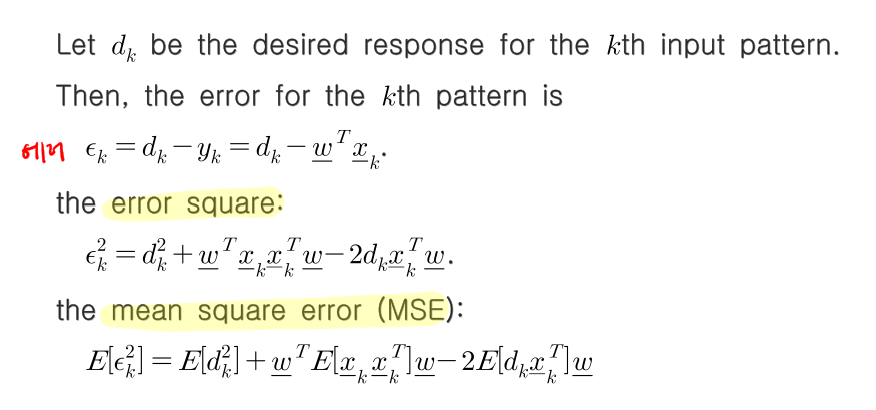
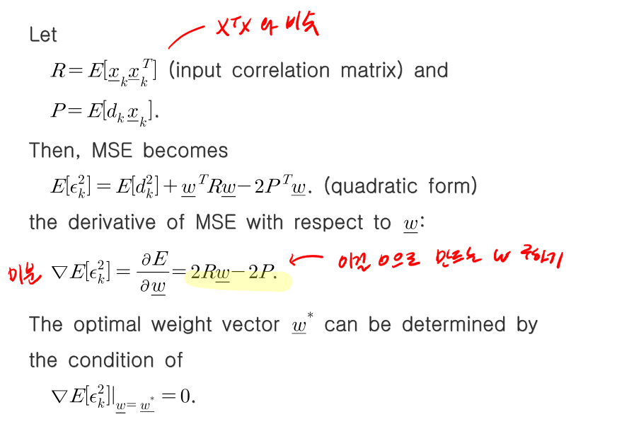
MMSE = E(dk^2) - P^T w* MSE = E(Ek^2) = E(dk^2) + w*Rw - 2p^Tw = MMSE + v^TRv
F(v) = v^TRv
이제 이 아이를 분석해야함.

gradient descent method (batch mode)

weight vector update rule을 만든다.
위에서 구한 R과 F(v)를 이용한다.

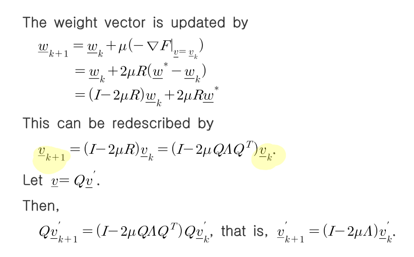
v’k+1 = (I-2MA)v’k (recursive equation)
v’k = (I-2MA)^kv0’
vk는 wk+1 - w* 이므로 v=0면 wk+1이 w* 즉 solution이 된다는것. 즉 I-2MA가 0이되도록만들어야함. M가 learning rate이므로 less than 1.
convergence condition이 0 < M < 1/tr[R]
이럴경우 MSE의 learning curve가 어떻게되는지 봐보자.
geomatric ratio : rn^2 = (I-2MA)^2
그래프로 그려보면 아래와같이 MMSE 위의 그래프모양을 그린다.

batch mode에서는 local minimum problem 빠지기쉽다.
on line mode는 빠져나오기쉽다. (더 선호됨)

least mean square (LMS) method (on-line mode)

delta hat이 unbiased estimator이다.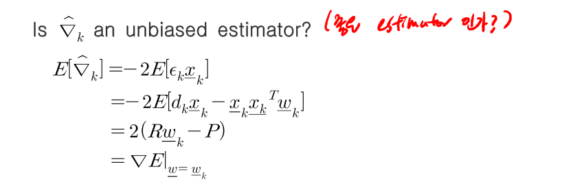
convergence condition이 0 < M < 1/tr[R]
–> online mode와 batch mode의 convergence condition이 똑같다.

check the performance of LMS

M = excess MSE / MMSE = E(MSE - MMSE) / MMSE (MMSE에비해 MSE가 얼마나 효율을냈는지 계산)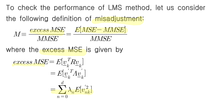
M = M*tr(R)

참고 https://blog.naver.com/61stu01/221274628848
https://blog.naver.com/mykepzzang/221568285099